Food science

At the beginning of June, I had the pleasure to attend my first conference about food science: The 7th International Symposium on Food Rheology and Structure.

I love food, my family loves food. With my sisters and brother we talk about food almost each time we meet. My aunts and uncles do the same. We love making food for each others and for our guests. My wife has the same kind of sensibility.

I love food, I love to cook. I love to improvise a new dish. I have dozens of spices in my kitchen, and I try to master their use, alone or in combination. I became versed in some recipes, likes lasagne bolognese, but I take on new challenges as often as possible. I often knead pasta or udon, I made chocolate éclair when they were impossible to find in Tokyo.

I love food, I love to understand it. My scientist brain can't be turned off when I cook. Mayonnaise is an emulsion, flour a granular material. When I make white sauce, the size of the eddies generated by my spoon is a visual indication of the Reynolds number and thus the viscosity of the sauce undergoing a sol-gel transition. Boiling water is a thermostat at 100°C.

I love food, I study it. My first independent project as an undergrad was about mayonnaise. Then I learned that soft matter science was a thing and went up to the PhD studying rather inedible soft materials. Freshly arrived in France as a postdoc, my new boss asked me if I wanted to study "waxy crude oil" or yoghurt. Of course I chose the later. I studied it as a physicist during 3 years and now finally I was able to present my results to food scientists.

I love food, but I am not a food scientist. I am not trying to formulate a new yoghurt. I don't make the link between the mouth feel adjectives rated by a panel of trained consumers and mechanical measurements. I am more interested by the physics that it reachable through the study of food systems.

I love food, and it was a pleasure to meet the food science community. I discovered very interesting systems, I heard interesting questions being raised, I received nice feedbacks about my contribution (see below). I even met a reader of this blog, hello Dilek!



I love food, I will meet this community again. I have been invited to Journées Scientifiques sur le thème Matière Molle pour la Science des Aliments, a conference to unite the French food science community. It will be held in October 28-29 in Montpellier.

CNRS position

After months of efforts, project writing and presentation rehearsals, I was selected to be hired as a CNRS researcher!

This permanent position starts in October and will be located in Institut Lumière et Matière (Light and Matter Institute) lab in Lyon University. I am so relieved to obtain a stable research position! Postdoc life is not bad but it lacks stability.

I am looking forward to join the new lab, but in the meanwhile I have stuff to do, especially now that I can focus back on science.

• get the paper about the wrinkling yoghurt accepted somewhere
• finish a paper pending since I left Tokyo 2 years and a half ago
• get rheological measurements done for the collaboration with next door chemists (can't talk about it, patent application pending)
• finalise minute understanding of yoghurt fracture and synaeresis by new confocal experiments

Because after that I will have to start my new project...

Multiscale localisation in 3D and confocal images deconvolution: Howto

Following last week's impulse, here is a tutorial about the subtleties of multiscale particle localisation from confocal 3D images.

For reference, this has been published as

A novel particle tracking method with individual particle size measurement and its application to ordering in glassy hard sphere colloids.

Leocmach, M., & Tanaka, H.

Soft Matter (2013), 9, 1447–1457.

doi:10.1039/c2sm27107a

ArXiV

The corresponding code is available at Sourceforge, including the IPython notebook corresponding to the present tutorial.

Particle localisation in a confocal image¶

First, import necessary library to load and display images

import numpy as np
from scipy.ndimage import gaussian_filter
from matplotlib import pyplot as plt
from colloids import track
%matplotlib inline

We also need to define functions to quickly display tracking results.

def draw_circles(xs, ys, rs, **kwargs):
    for x,y,r in zip(xs,ys,rs):
        circle = plt.Circle((x,y), radius=r, **kwargs)
        plt.gca().add_patch(circle)
        
def display_cuts(imf, centers, X=30, Y=25, Z=30):
    """Draw three orthogonal cuts with corresponding centers"""
    plt.subplot(1,3,1);
    draw_circles(centers[:,0], centers[:,1], centers[:,-2], facecolor='none', edgecolor='g')
    plt.imshow(imf[Z], 'hot',vmin=0,vmax=255);
    plt.subplot(1,3,2);
    draw_circles(centers[:,0], centers[:,2], centers[:,-2], facecolor='none', edgecolor='g')
    plt.imshow(imf[:,Y], 'hot',vmin=0,vmax=255);
    plt.subplot(1,3,3);
    draw_circles(centers[:,1], centers[:,2], centers[:,-2], facecolor='none', edgecolor='g')
    plt.imshow(imf[:,:,X], 'hot',vmin=0,vmax=255);

Raw confocal image¶

Load the test data, which is only a detail of a full 3D stack. Display different cuts.

Note that raw confocal images are heavily distorted in the \(z\) direction. We actually have 4 particles in the image: two small on top of each other, one on the side and a slightly larger below and on the side.

imf = np.fromfile('../../../multiscale/test_input/Z_elong.raw', dtype=np.uint8).reshape((55,50,50))
plt.subplot(1,3,1).imshow(imf[30], 'hot',vmin=0,vmax=255);
plt.subplot(1,3,2).imshow(imf[:,25], 'hot',vmin=0,vmax=255);
plt.subplot(1,3,3).imshow(imf[:,:,30], 'hot',vmin=0,vmax=255);

Create a finder object of the same shape as the image. Seamlessly work with 3D images.

finder = track.MultiscaleBlobFinder(imf.shape, Octave0=False, nbOctaves=4)

Feed the image in the tracker with default tracking parameters. The output has four columns : \((x,y,z,r,i)\) where \(r\) is a first approximation of the radius of the particle (see below) and \(i\) is a measure of the brightness of the particle.

centers = finder(imf)
print centers.shape
print "smallest particle detected has a radius of %g px"%(centers[:,-2].min()) 
display_cuts(imf, centers)

(2, 5)
smallest particle detected has a radius of 4.40672 px

This is a pretty bad job. Only two particle detected correctly. The top and side small particles are not detected.

Let us try not to remove overlapping.

centers = finder(imf, removeOverlap=False)
print centers.shape
print "smallest particle detected has a radius of %g px"%(centers[:,-2].min()) 
display_cuts(imf, centers)

(4, 5)
smallest particle detected has a radius of 4.40672 px

Now we have all the particles.

We have two effects at play here that fool the overlap removal: - The radii guessed by the algorithm are too large. - The particles aligned along \(z\) are localised too close together.

Both effects are due to the elongation in \(z\).

Simple deconvolution of a confocal image¶

The image \(y\) acquired by a microscope can be expressed as

\(y = x \star h + \epsilon,\)

where \(\star\) is the convolution operator, \(x\) is the perfect image, \(h\) is the point spread function (PSF) of the microscope and \(\epsilon\) is the noise independent of both \(x\) and \(h\). The process of estimating \(x\) from \(y\) and some theoretical or measured expression of \(h\) is called deconvolution. Deconvolution in the presence of noise is a difficult problem. Hopefully here we do not need to reconstruct the original image, but only our first Gaussian blurred version of it. Indeed, after a reasonable amount of blur in three dimensions, the noise can be neglected and we thus obtain:

\(y_0 \approx G_0 \star h,\)

or in Fourier space

\(\mathcal{F}[y_0] = \mathcal{F}[G_0] \times \mathcal{F}[h].\)

Once \(\mathcal{F}[h]\) is known the deconvolution reduces to a simple division in Fourier space.

Measuring the kernel¶

\(\mathcal{F}[h]\) should be measured in an isotropic system and in the same conditions (magnification, number of pixels, indices of refraction, etc.) as the experiment of interest.

Since a 3D image large enough to be isotropic is too big to share in an example, I just use the image of interest. Don't do this at home.

imiso = np.fromfile('../../../multiscale/test_input/Z_elong.raw', dtype=np.uint8).reshape((55,50,50))
kernel = track.get_deconv_kernel(imiso)
plt.plot(kernel);

The kernel variable here is actually \(1/\mathcal{F}[h]\)

Kernel test¶

What not to do: deconvolve the unblurred image.

imd = track.deconvolve(imf, kernel)
plt.subplot(1,3,1).imshow(imd[30], 'hot',vmin=0,vmax=255);
plt.subplot(1,3,2).imshow(imd[:,25], 'hot',vmin=0,vmax=255);
plt.subplot(1,3,3).imshow(imd[:,:,30], 'hot',vmin=0,vmax=255);

Noisy isn't it? Yet we have saturated the color scale between 0 and 255, otherwise artifacts would be even more apparent.

What the program will actually do: deconvolved the blurred image.

imb = gaussian_filter(imf.astype(float), 1.6)
plt.subplot(1,3,1).imshow(imb[30], 'hot',vmin=0,vmax=255);
plt.subplot(1,3,2).imshow(imb[:,25], 'hot',vmin=0,vmax=255);
plt.subplot(1,3,3).imshow(imb[:,:,30], 'hot',vmin=0,vmax=255);

imbd = track.deconvolve(imb, kernel)
plt.subplot(1,3,1).imshow(imbd[30], 'hot',vmin=0,vmax=255);
plt.subplot(1,3,2).imshow(imbd[:,25], 'hot',vmin=0,vmax=255);
plt.subplot(1,3,3).imshow(imbd[:,:,30], 'hot',vmin=0,vmax=255);

The way the noise is amplified by deconvolution is obvious when we compare the histograms of the 4 versions of the image.

for i, (l, im) in enumerate(zip(['raw', 'blurred', 'deconv', 'blur deconv'], [imf, imb, imd, imbd])):
    plt.plot(
             np.arange(-129,363,8), 
             np.histogram(im, np.arange(-129,371,8))[0]*10**i, 
             label=l+' (%d,%d)'%(im.min(), im.max()));
plt.xlim(-130,360);
plt.yscale('log');
plt.legend(loc='upper right');

Obviously negative values should be discarded, and will be discarded by the algorithm.

Localisation using deconvolved image¶

Not removing the overlaping particles, we use the deconvolution kernel.

reload(track)
centers = finder(imf, removeOverlap=False, deconvKernel=kernel)
print centers.shape
print "smallest particle detected has a radius of %g px"%(centers[:,-2].min()) 
display_cuts(imf, centers)

(5, 5)
smallest particle detected has a radius of 3.79771 px

All particles are found and actually they are not overlaping. However we got a spurious detection, probably some noise that got amplified by the deconvolution. It is easily removed by a threshold in intensity.

print centers

[[ 16.31334384  44.07373885  21.50444345   3.79770755  -0.37019082]
 [ 26.79860906  22.0435863   21.89833819   3.89324706 -15.95536745]
 [ 26.92095001  21.83422163  32.72685299   3.85903411 -17.3271687 ]
 [ 26.11610631  31.30829898  36.11323148   4.33867807 -21.06731591]
 [ 31.77923381  26.78655827  44.05564076   4.03334069 -20.1763175 ]]

centers = centers[centers[:,-1]<-1]
display_cuts(imf, centers)

We can also display the results with respect to the blurred and deconvolved version of the image that we can find by introspection.

display_cuts(finder.octaves[1].layersG[0], centers)

From scales to sizes¶

This is pretty much like in 2D.

In [17]:

from colloids.particles import get_bonds
s = track.radius2sigma(centers[:,-2], dim=3)
bonds, dists = get_bonds(positions=centers[:,:-2], radii=centers[:,-2], maxdist=3.0)
brights1 = track.solve_intensities(s, bonds, dists, centers[:,-1])
radii1 = track.global_rescale_intensity(s, bonds, dists, brights1)
centers2 = np.copy(centers)
centers2[:,-2] = radii1
display_cuts(imf, centers2)

Multiscale localisation in 2D: Howto

My multiscale tracking algorithm has been out for 3 years, published, on ArXiV. However, its availability at Sourceforge has been theoretical, since I never wrote a proper tutorial on how to use the code.

Today's post is an attempt is this direction. I will explain how to localise and size particles on a 2D image using the Python implementation of the algorithm. This is also one of my first attempt to use ipython notebooks and to export them on this blog. You can find the original notebook in the sourceforge repository (/trunc/python/colloids/notebooks/).

Prerequisites are the python code imported from the repository, in your PYTHONPATH. You will probably need a few other packages (python-bs4, libboost-all-dev, python-numexpr) and a working C++ compiler (GCC or MINGW on Windows). Of course, python 2.?, numpy, ipython are needed. If you don't know what ipython is, and you are interested in my code, then you should learn about it.

First, import necessary library to load and display images

import numpy as np
from matplotlib import pyplot as plt
from colloids import track
%matplotlib inline

We also need to define a function to quickly plot circles of different sizes on a figure

def draw_circles(xs, ys, rs, **kwargs):
    for x,y,r in zip(xs,ys,rs):
        circle = plt.Circle((x,y), radius=r, **kwargs)
        plt.gca().add_patch(circle)

Load a picture containing bright particles on a dark background and immediatly display this image in a figure

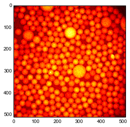
im = plt.imread('droplets.jpg')
plt.imshow(im, 'hot');
plt.show()

Create a finder object of the same shape as the image. This actually creates many sub-finder objects, one for each \Octave\. Octave 1 has the same shape as the image. Octave 2 is twice smaller. Octave 3 is four time smaller than Octave 1, etc. Optionally, you can create Octave 0 that is twice bigger than Octave 1, but it takes a lot of memory and tracking results are bad. So here we set Octave0=False. The maximal scale at which particles are looked for is set by nbOctaves.

finder = track.MultiscaleBlobFinder(im.shape, Octave0=False, nbOctaves=4)
finder?

Feed the image in the tracker with default tracking parameters already does a great job. the output has three columns : \((x,y,r,i)\) where \(r\) is a first approximation of the radius of the particle (see below) and \(i\) is a measure of the brightness of the particle.

The smallest particle that can be detected with the default parameter \(k=1.6\) in 2D is about 3 pixels in radius. In 3D it would be 4 pixels in radius. To increase this smallest scale you can increase the parameter \(k\). Decreasing \(k\) below 1.2 is probably not a good idear since you will detect noise as particles. Redo your acquisition with higher resolution instead.

centers = finder(im, k=1.6)
print centers.shape
print "smallest particle detected has a radius of %g px"%(centers[:,-2].min()) 
draw_circles(centers[:,0], centers[:,1], centers[:,2], facecolor='none', edgecolor='g')
plt.imshow(im, 'hot');

(305, 4)
smallest particle detected has a radius of 0.00130704 px

However some small particles are missing, for example near the large particle at the center. Maybe it is because by default the MultiscaleFinder removes overlapping particles? Let us try to disable this removal.

centers = finder(im, removeOverlap=False)
draw_circles(centers[:,0], centers[:,1], centers[:,2], facecolor='none', edgecolor='g')
plt.imshow(im, 'hot');

Well, we gained only spurious detections.

We can also try to disable a filter that rejects local minima that are elongated in space.

centers = finder(im, maxedge=-1)
draw_circles(centers[:,0], centers[:,1], centers[:,2], facecolor='none', edgecolor='g')
plt.imshow(im, 'hot');

For sanity, it is probably better to filter out the particles with a radius smaller than 1 pixel.

centers = centers[centers[:,-2]>1]

Introspection¶

The intermediate steps of the algorithm are accessible. For example one can access the octaves (lines in figure below) and their successively blured versions of the original image.

#get maximum intensity to set color bar
m = max([oc.layersG.max() for oc in finder.octaves[1:]])
for o, oc in enumerate(finder.octaves[1:]):
    for l, lay in enumerate(oc.layersG):
        a = plt.subplot(len(finder.octaves)-1,len(oc.layersG),len(oc.layersG)*o + l +1)
        #hide ticks for clarity
        a.axes.get_xaxis().set_visible(False)
        a.axes.get_yaxis().set_visible(False)
        plt.imshow(lay, 'hot', vmin=0, vmax=m);
        

One can also access the difference of Gaussians. Here relevant values are negative, so we inverse the colors and saturate at zero.

#get maximum intensity to set color bar
m = min([oc.layers.min() for oc in finder.octaves[1:]])
for o, oc in enumerate(finder.octaves[1:]):
    for l, lay in enumerate(-oc.layers):
        a = plt.subplot(len(finder.octaves)-1,len(oc.layers),len(oc.layers)*o + l +1)
        #hide ticks for clarity
        a.axes.get_xaxis().set_visible(False)
        a.axes.get_yaxis().set_visible(False)
        plt.imshow(lay, 'hot', vmin=0, vmax=-m);
        

Each OctaveFinder looks for local minima (very negative) in the difference of Gaussians space. Local minima in understood relative to space \((x,y)\) and scale \(s\). The job of the MultiscaleFinder is to coordinate the action of the Octaves to return a coherent result.

From scales to sizes¶

The multiscale algorithm finds local minima in space and scale \(s\). How can we convert scales in actual sizes (particle radius \(r\))? If the particles are far apart, their respective spots do not overlap, so we can use the formula

\(R = s \sqrt{\frac{2d\ln \alpha}{1-\alpha^{-2}}}\)

where \(d\) is the dimensionality of the image (here 2) and \(\alpha=2^{1/n}\) with \(n\) the number of subdivisions in an octave (parameter nbLayers when creating the MultiscaleFinder).

MultiscaleFinder actually does this conversion when returning its result.

But what if particles are close together? Then their respective spots overlap and the scale in only indirectly related to the size. We need to take into account the distance between particles and their relative brightnesses. The first step is to revert to scales.

s = track.radius2sigma(centers[:,-2], dim=2)

Then we have to find the couples of particles whoes spots probably overlap. The submodule colloids.particles has a function to do this. On a large system, this is the most costly function.

In [13]:

from colloids.particles import get_bonds
bonds, dists = get_bonds(positions=centers[:,:-2], radii=centers[:,-2], maxdist=3.0)

Now we have all the ingredients to run the reconstruction.

Note: You need boost libraries installed on your system to proceed.

sudo apt-get install libboost-all-dev

First, we will obtain the brightness of each particle form the value of the Difference of Gaussians at the place and scale of every particle, e.g. the last column of centers.

In [14]:

brights1 = track.solve_intensities(s, bonds, dists, centers[:,-1])

Second, we use these brightnesses to obtain the new radii.

In [15]:

radii1 = track.global_rescale_intensity(s, bonds, dists, brights1)
draw_circles(centers[:,0], centers[:,1], radii1, facecolor='none', edgecolor='g')
plt.imshow(im, 'hot');

The radii were underestimated indeed!

histR0, bins = np.histogram(centers[:,-2], bins=np.arange(30))
histR1, bins = np.histogram(radii1, bins=np.arange(30))
plt.step(bins[:-1], histR0, label='supposed dilute');
plt.step(bins[:-1], histR1, label='corrected for overlap');
plt.xlabel('radius (px)');
plt.ylabel('count');
plt.legend(loc='upper right');

It is always possible to iterate first and second steps above.

In [17]:

brights2 = track.solve_intensities(s, bonds, dists, centers[:,-1], R0=radii1)
radii2 = track.global_rescale_intensity(s, bonds, dists, brights, R0=radii1)
draw_circles(centers[:,0], centers[:,1], radii2, facecolor='none', edgecolor='g')
plt.imshow(im, 'hot');

In [18]:

histR2, bins = np.histogram(radii2, bins=np.arange(30))
plt.step(bins[:-1], histR0, label='supposed dilute');
plt.step(bins[:-1], histR1, label='corrected for overlap');
plt.step(bins[:-1], histR2, label='second iteration');
plt.xlabel('radius (px)');
plt.ylabel('count');
plt.legend(loc='upper right');

But most of the times it does not help much.

EnDirectDuLabo = RealScientists.fr

Two weeks ago I owned the Twitter account @EnDirectDuLabo. For those who know RealScientists, it is the French version. For those who don't, it is researchers taking turns to stir a Twitter account and tell what is the everyday life of a real scientist.

Somehow this is the same ideal I intended for this blog. However Twitter format makes it easier. In 140 characters you can't explain your research deep enough to bother your reader. You have to be clear with your idears, one at the time. Punchlines and soundbites.

If you read French, here is the storify of my week: