I am using IPython a lot, either as a command prompt or in a Jupyter notebook. This is great to analyse data on the go. During such analysis you may generate some files, either some intermediate data, or figures.
Sometimes, weeks, months or years later you would like to remember exactly what you did to generate this file. This is important for science reproducibility, to check you followed the right method or just to reuse this handy bit of code.
When you have copied the code in a script file, easy. When you have organised properly your notebook and never delete the interesting cell, piece of cake. When it was yesterday and you can press the up key N times to look for the right set of lines in the history, painful but doable. But this no warranty, no rigorous method. One day you will think that writing the script is useless, one day you will delete the wrong cell in your notebook, and months after you will have to come back to this analysis and the history will be gone.
It is really akin to the lab notebook, the one in which you note the date, the temperature, the sample name, the procedure you follow, the result of the measures and all the qualitative observations. Some of it seems to matter much at the moment, but if you forget to write it down, you will never be able to reproduce your experiment.
How to make IPython generate this virtual notebook for you?
You want a file per IPython session with all the commands you type. You can achieve this manually by typing at the begining of each session
%logstart mylogfile append
But of course, you will forget.
We have to make this automatic. This is made possible by the profile configuration of IPython. If you have never created a profile for IPython, type in a terminal
ipython profile create
This will generate a default profile in HOME/.ipython/profile_default
Edit the file HOME/.ipython/profile_default/ipython_config.py and look for the line #c.InteractiveShell.logappend = ''
Instead, write the following lines
import os
from time import strftime
ldir = os.path.join(os.path.expanduser("~"),'.ipython')
filename = os.path.join(ldir, strftime('%Y-%m-%d_%H-%M')+".py")
notnew = os.path.exists(filename)
with open(filename,'a') as file_handle:
if notnew:
file_handle.write("# =================================")
else:
file_handle.write("#!/usr/bin/env python \n# %s.py \n"
"# IPython automatic logging file" %
strftime('%Y-%m-%d'))
file_handle.write("# %s \n# =================================" %
strftime('%H:%M'))
# Start logging to the given file in append mode. Use `logfile` to specify a log
# file to **overwrite** logs to.
c.InteractiveShell.logappend = filename
And here you are, each time you open a IPython session, either console or notebook, a file is created in HOME/.ipython. The name of this file contains the date and time of the opening of the session (format YYYY-MM-DD_hh-mm). Everything you type during this session will be written automatically in this file.
The good news first: our paper on wrinkling yoghurt was accepted. I won't tell you where since it is under embargo. If you want to know what it means to have a paper accepted, and what sort of work in involved (disclaimer: comparable to the amount of work need for the research in itself), have a look at this:
But last Friday night, 11pm, we received a mail from the editorial office saying something like
Our typesetting department must have Word document files of your paper [...].
Please provide these files as Word documents as quickly as possible and within the next 8 hours to keep your paper on schedule for publication.
Well, except for the short notice and the looming weekend, there was a big problem. Our paper was not a Word file and the conversion is all but easy. Let me explain
Academic paper formatting
But there is another last step not described here: formatting. Of course, you can open any text editor (notepad, your webmail) and type words after words to write the text of your article. But then, you would miss:
figures
equations
cross-references
Figures are the graphs, the pictures and the drawings. You can insert them if you switch to any modern word processor, LibreOffice or Microsoft Word for example. Getting them beautiful and right is a work in itself.
Equations are a nightmare with Word. Just writing y≈αx7 makes you seek in 3-4 different menus. But you can do it. Markup languages, like the HTML of this page, makes it easier once you know the syntax. LaTeX is a markup language made for equations. The above equation just writes $y=\alpha x^7$. LaTeX syntax for equations has become a de facto standard, so other languages likes Markup, offer to write the math parts in LaTeX. Plugins in LibreOffice also do that.
Cross referencing means that in your text you can write "see Figure 3", then switch figures 3 and 4 and have "see Figure 4" written automatically in your text. In practice you do not write the figure number, but insert a reference that the program will convert into the figure number. You can do that with Word through one menu and a rather unhelpful dialogue box. In LaTeX it is just "Figure \ref{fig:velocitygraph}". Actually, in the final document, you can even get an hyperlink to the figure. Same with chapters, sections, equations.
What is great with LaTeX is that your bibliography can be generated the same way. You just insert "was discovered recently \cite{Leocmach2015}" and the paper Leocmach2015 gets inserted in your bibliography, formatted properly and consistently. In the final document you would get "was discovered recently [17]" with an hyperlink going to the 17th item in your bibliography. Of course, you have ways to do that with plugins in Word or LibreOffice.
LaTeX is also nice because you can specify what you mean and then let the program format it for you. For example, when I want to write "10 µm" what I mean is ten micro metre, not "one zero space greek letter mu m", so in LaTeX I write "\SI{10}{\micro\metre}" and it will generate a "10", followed by an unbreakable space (you don't want the number and the unit on different lines or pages), followed by a micro sign µ (different from the μ in some fonts) and a "m".
By the way, LaTeX is open source and free, no need for a licence. The "final document" is a PDF that anybody can read. Actually, until Friday night Editors and Referees of our paper had only seen and judged the PDF. Nobody was caring about formatting (even if it helps to have a clean looking paper to show rather than a messy Word file).
So LaTeX is made for academic paper writing, and heavily used in Math, Physics and other communities. It would be unthinkable that a journal specialised in Physics refuse LaTeX formatted paper. However for Biology, Word is the norm. It must be a pain for the typesetting departments who have to translate Word format into something more usable. Broad audience journals often accept both, but not the journal we submitted to.
Latex to Word conversion
I spent most of my Saturday thinking about a reliable and reusable way to convert my paper. This won't be the last time I am asked to provide a Word file. I received advices on Twitter, tried various solutions, all unsatisfactory, and at the end I settled to this method:
Dumb down the LaTeX layout. I was using a two column layout with figures within the text, I switched to a single column layout with a figure per page at the end of the document.
Add \usepackage{times} to your LaTeX preamble in order to use Word default font Times New Roman.
Let LaTeX make the PDF. All the commands, custom packages, etc. are taken into account. Cross references and bibliography are also right.
Convert PDF into Word. @fxcouder did it for me using Adobe. There are probably open source ways of doing it. Simple equations were preserved, but as soon as fractions were involved the format was messy.
Clean the Word file. No messing up, you need a real Microsoft Word with a licence. Work in 97/2000 compatibility mode. You need to show formatting marks, track down and delete the section breaks to obtain a single flow of text. Fix also the line breaks and hyphenations for the paragraphs to be in one piece. All messy equations must be cleaned up, leaving only the numbering for the numbered ones.
Re type the equations. I did this by hand in Word since I had few equations to retype.
Copy the whole text and paste in into the template provided by the editor.
Rather than retyping the equations, an other way would be to process the original tex document into an ODT (LibreOffice) document using pandoc.
pandoc -s article.tex -o article.odt
Pandoc is messing cross-references, citations and anything custom in your LaTeX code. Do not use it for the conversion of the main text. However it gets the equations right. Then from LibreOffice, you can export the equations and import them back into the Word document.
So, why worry? It takes you only half a day for a 15 pages paper instead of the 8 hours requested by the editorial office.
I love food, my family loves food. With my sisters and brother we talk about food almost each time we meet. My aunts and uncles do the same. We love making food for each others and for our guests. My wife has the same kind of sensibility.
I love food, I love to cook. I love to improvise a new dish. I have dozens of spices in my kitchen, and I try to master their use, alone or in combination. I became versed in some recipes, likes lasagne bolognese, but I take on new challenges as often as possible. I often knead pasta or udon, I made chocolate éclair when they were impossible to find in Tokyo.
I love food, I love to understand it. My scientist brain can't be turned off when I cook. Mayonnaise is an emulsion, flour a granular material. When I make white sauce, the size of the eddies generated by my spoon is a visual indication of the Reynolds number and thus the viscosity of the sauce undergoing a sol-gel transition. Boiling water is a thermostat at 100°C.
I love food, I study it. My first independent project as an undergrad was about mayonnaise. Then I learned that soft matter science was a thing and went up to the PhD studying rather inedible soft materials. Freshly arrived in France as a postdoc, my new boss asked me if I wanted to study "waxy crude oil" or yoghurt. Of course I chose the later. I studied it as a physicist during 3 years and now finally I was able to present my results to food scientists.
I love food, but I am not a food scientist. I am not trying to formulate a new yoghurt. I don't make the link between the mouth feel adjectives rated by a panel of trained consumers and mechanical measurements. I am more interested by the physics that it reachable through the study of food systems.
I love food, and it was a pleasure to meet the food science community. I discovered very interesting systems, I heard interesting questions being raised, I received nice feedbacks about my contribution (see below). I even met a reader of this blog, hello Dilek!
After months of efforts, project writing and presentation rehearsals, I was selected to be hired as a CNRS researcher!
This permanent position starts in October and will be located in Institut Lumière et Matière (Light and Matter Institute) lab in Lyon University. I am so relieved to obtain a stable research position! Postdoc life is not bad but it lacks stability.
I am looking forward to join the new lab, but in the meanwhile I have stuff to do, especially now that I can focus back on science.
get the paper about the wrinkling yoghurt accepted somewhere
finish a paper pending since I left Tokyo 2 years and a half ago
get rheological measurements done for the collaboration with next door chemists (can't talk about it, patent application pending)
finalise minute understanding of yoghurt fracture and synaeresis by new confocal experiments
Because after that I will have to start my new project...
We also need to define functions to quickly display tracking results.
defdraw_circles(xs,ys,rs,**kwargs):forx,y,rinzip(xs,ys,rs):circle=plt.Circle((x,y),radius=r,**kwargs)plt.gca().add_patch(circle)defdisplay_cuts(imf,centers,X=30,Y=25,Z=30):"""Draw three orthogonal cuts with corresponding centers"""plt.subplot(1,3,1);draw_circles(centers[:,0],centers[:,1],centers[:,-2],facecolor='none',edgecolor='g')plt.imshow(imf[Z],'hot',vmin=0,vmax=255);plt.subplot(1,3,2);draw_circles(centers[:,0],centers[:,2],centers[:,-2],facecolor='none',edgecolor='g')plt.imshow(imf[:,Y],'hot',vmin=0,vmax=255);plt.subplot(1,3,3);draw_circles(centers[:,1],centers[:,2],centers[:,-2],facecolor='none',edgecolor='g')plt.imshow(imf[:,:,X],'hot',vmin=0,vmax=255);
Load the test data, which is only a detail of a full 3D stack. Display different cuts.
Note that raw confocal images are heavily distorted in the \(z\) direction. We actually have 4 particles in the image: two small on top of each other, one on the side and a slightly larger below and on the side.
Feed the image in the tracker with default tracking parameters. The output has four columns : \((x,y,z,r,i)\) where \(r\) is a first approximation of the radius of the particle (see below) and \(i\) is a measure of the brightness of the particle.
centers=finder(imf)printcenters.shapeprint"smallest particle detected has a radius of %g px"%(centers[:,-2].min())display_cuts(imf,centers)
(2, 5)
smallest particle detected has a radius of 4.40672 px
This is a pretty bad job. Only two particle detected correctly. The top and side small particles are not detected.
Let us try not to remove overlapping.
centers=finder(imf,removeOverlap=False)printcenters.shapeprint"smallest particle detected has a radius of %g px"%(centers[:,-2].min())display_cuts(imf,centers)
(4, 5)
smallest particle detected has a radius of 4.40672 px
Now we have all the particles.
We have two effects at play here that fool the overlap removal: - The radii guessed by the algorithm are too large. - The particles aligned along \(z\) are localised too close together.
The image \(y\) acquired by a microscope can be expressed as
\(y = x \star h + \epsilon,\)
where \(\star\) is the convolution operator, \(x\) is the perfect image, \(h\) is the point spread function (PSF) of the microscope and \(\epsilon\) is the noise independent of both \(x\) and \(h\). The process of estimating \(x\) from \(y\) and some theoretical or measured expression of \(h\) is called deconvolution. Deconvolution in the presence of noise is a difficult problem. Hopefully here we do not need to reconstruct the original image, but only our first Gaussian blurred version of it. Indeed, after a reasonable amount of blur in three dimensions, the noise can be neglected and we thus obtain:
\(\mathcal{F}[h]\) should be measured in an isotropic system and in the same conditions (magnification, number of pixels, indices of refraction, etc.) as the experiment of interest.
Since a 3D image large enough to be isotropic is too big to share in an example, I just use the image of interest. Don't do this at home.
Not removing the overlaping particles, we use the deconvolution kernel.
reload(track)centers=finder(imf,removeOverlap=False,deconvKernel=kernel)printcenters.shapeprint"smallest particle detected has a radius of %g px"%(centers[:,-2].min())display_cuts(imf,centers)
(5, 5)
smallest particle detected has a radius of 3.79771 px
All particles are found and actually they are not overlaping. However we got a spurious detection, probably some noise that got amplified by the deconvolution. It is easily removed by a threshold in intensity.
My multiscale tracking algorithm has been out for 3 years, published, on ArXiV. However, its availability at Sourceforge has been theoretical, since I never wrote a proper tutorial on how to use the code.
Today's post is an attempt is this direction. I will explain how to localise and size particles on a 2D image using the Python implementation of the algorithm. This is also one of my first attempt to use ipython notebooks and to export them on this blog. You can find the original notebook in the sourceforge repository (/trunc/python/colloids/notebooks/).
Prerequisites are the python code imported from the repository, in your PYTHONPATH. You will probably need a few other packages (python-bs4, libboost-all-dev, python-numexpr) and a working C++ compiler (GCC or MINGW on Windows). Of course, python 2.?, numpy, ipython are needed. If you don't know what ipython is, and you are interested in my code, then you should learn about it.
First, import necessary library to load and display images
Create a finder object of the same shape as the image. This actually creates many sub-finder objects, one for each \Octave\. Octave 1 has the same shape as the image. Octave 2 is twice smaller. Octave 3 is four time smaller than Octave 1, etc. Optionally, you can create Octave 0 that is twice bigger than Octave 1, but it takes a lot of memory and tracking results are bad. So here we set Octave0=False. The maximal scale at which particles are looked for is set by nbOctaves.
Feed the image in the tracker with default tracking parameters already does a great job. the output has three columns : \((x,y,r,i)\) where \(r\) is a first approximation of the radius of the particle (see below) and \(i\) is a measure of the brightness of the particle.
The smallest particle that can be detected with the default parameter \(k=1.6\) in 2D is about 3 pixels in radius. In 3D it would be 4 pixels in radius. To increase this smallest scale you can increase the parameter \(k\). Decreasing \(k\) below 1.2 is probably not a good idear since you will detect noise as particles. Redo your acquisition with higher resolution instead.
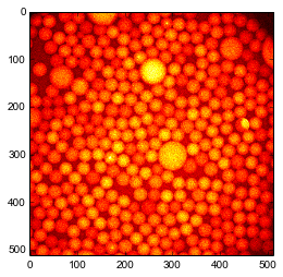
centers=finder(im,k=1.6)printcenters.shapeprint"smallest particle detected has a radius of %g px"%(centers[:,-2].min())draw_circles(centers[:,0],centers[:,1],centers[:,2],facecolor='none',edgecolor='g')plt.imshow(im,'hot');
(305, 4)
smallest particle detected has a radius of 0.00130704 px
However some small particles are missing, for example near the large particle at the center. Maybe it is because by default the MultiscaleFinder removes overlapping particles? Let us try to disable this removal.
The intermediate steps of the algorithm are accessible. For example one can access the octaves (lines in figure below) and their successively blured versions of the original image.
#get maximum intensity to set color barm=max([oc.layersG.max()forocinfinder.octaves[1:]])foro,ocinenumerate(finder.octaves[1:]):forl,layinenumerate(oc.layersG):a=plt.subplot(len(finder.octaves)-1,len(oc.layersG),len(oc.layersG)*o+l+1)#hide ticks for claritya.axes.get_xaxis().set_visible(False)a.axes.get_yaxis().set_visible(False)plt.imshow(lay,'hot',vmin=0,vmax=m);
One can also access the difference of Gaussians. Here relevant values are negative, so we inverse the colors and saturate at zero.
#get maximum intensity to set color barm=min([oc.layers.min()forocinfinder.octaves[1:]])foro,ocinenumerate(finder.octaves[1:]):forl,layinenumerate(-oc.layers):a=plt.subplot(len(finder.octaves)-1,len(oc.layers),len(oc.layers)*o+l+1)#hide ticks for claritya.axes.get_xaxis().set_visible(False)a.axes.get_yaxis().set_visible(False)plt.imshow(lay,'hot',vmin=0,vmax=-m);
Each OctaveFinder looks for local minima (very negative) in the difference of Gaussians space. Local minima in understood relative to space \((x,y)\) and scale \(s\). The job of the MultiscaleFinder is to coordinate the action of the Octaves to return a coherent result.
The multiscale algorithm finds local minima in space and scale \(s\). How can we convert scales in actual sizes (particle radius \(r\))? If the particles are far apart, their respective spots do not overlap, so we can use the formula
\(R = s \sqrt{\frac{2d\ln \alpha}{1-\alpha^{-2}}}\)
where \(d\) is the dimensionality of the image (here 2) and \(\alpha=2^{1/n}\) with \(n\) the number of subdivisions in an octave (parameter nbLayers when creating the MultiscaleFinder).
MultiscaleFinder actually does this conversion when returning its result.
But what if particles are close together? Then their respective spots overlap and the scale in only indirectly related to the size. We need to take into account the distance between particles and their relative brightnesses. The first step is to revert to scales.
s=track.radius2sigma(centers[:,-2],dim=2)
Then we have to find the couples of particles whoes spots probably overlap. The submodule colloids.particles has a function to do this. On a large system, this is the most costly function.
Now we have all the ingredients to run the reconstruction.
Note: You need boost libraries installed on your system to proceed.
sudo apt-get install libboost-all-dev
First, we will obtain the brightness of each particle form the value of the Difference of Gaussians at the place and scale of every particle, e.g. the last column of centers.