Sunday, February 22, 2015

Multiscale localisation in 2D: Howto


My multiscale tracking algorithm has been out for 3 years, published, on ArXiV. However, its availability at Sourceforge has been theoretical, since I never wrote a proper tutorial on how to use the code.


Today's post is an attempt is this direction. I will explain how to localise and size particles on a 2D image using the Python implementation of the algorithm. This is also one of my first attempt to use ipython notebooks and to export them on this blog. You can find the original notebook in the sourceforge repository (/trunc/python/colloids/notebooks/).


Prerequisites are the python code imported from the repository, in your PYTHONPATH. You will probably need a few other packages (python-bs4, libboost-all-dev, python-numexpr) and a working C++ compiler (GCC or MINGW on Windows). Of course, python 2.?, numpy, ipython are needed. If you don't know what ipython is, and you are interested in my code, then you should learn about it.


First, import necessary library to load and display images

import numpy as np
from matplotlib import pyplot as plt
from colloids import track
%matplotlib inline


We also need to define a function to quickly plot circles of different sizes on a figure

def draw_circles(xs, ys, rs, **kwargs):
    for x,y,r in zip(xs,ys,rs):
        circle = plt.Circle((x,y), radius=r, **kwargs)
        plt.gca().add_patch(circle)


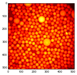
Load a picture containing bright particles on a dark background and immediatly display this image in a figure

im = plt.imread('droplets.jpg')
plt.imshow(im, 'hot');
plt.show()


Create a finder object of the same shape as the image. This actually creates many sub-finder objects, one for each \Octave\. Octave 1 has the same shape as the image. Octave 2 is twice smaller. Octave 3 is four time smaller than Octave 1, etc. Optionally, you can create Octave 0 that is twice bigger than Octave 1, but it takes a lot of memory and tracking results are bad. So here we set Octave0=False. The maximal scale at which particles are looked for is set by nbOctaves.

finder = track.MultiscaleBlobFinder(im.shape, Octave0=False, nbOctaves=4)
finder?


Feed the image in the tracker with default tracking parameters already does a great job. the output has three columns : \((x,y,r,i)\) where \(r\) is a first approximation of the radius of the particle (see below) and \(i\) is a measure of the brightness of the particle.

The smallest particle that can be detected with the default parameter \(k=1.6\) in 2D is about 3 pixels in radius. In 3D it would be 4 pixels in radius. To increase this smallest scale you can increase the parameter \(k\). Decreasing \(k\) below 1.2 is probably not a good idear since you will detect noise as particles. Redo your acquisition with higher resolution instead.

centers = finder(im, k=1.6)
print centers.shape
print "smallest particle detected has a radius of %g px"%(centers[:,-2].min()) 
draw_circles(centers[:,0], centers[:,1], centers[:,2], facecolor='none', edgecolor='g')
plt.imshow(im, 'hot');


(305, 4)
smallest particle detected has a radius of 0.00130704 px


However some small particles are missing, for example near the large particle at the center. Maybe it is because by default the MultiscaleFinder removes overlapping particles? Let us try to disable this removal.

centers = finder(im, removeOverlap=False)
draw_circles(centers[:,0], centers[:,1], centers[:,2], facecolor='none', edgecolor='g')
plt.imshow(im, 'hot');


Well, we gained only spurious detections.

We can also try to disable a filter that rejects local minima that are elongated in space.

centers = finder(im, maxedge=-1)
draw_circles(centers[:,0], centers[:,1], centers[:,2], facecolor='none', edgecolor='g')
plt.imshow(im, 'hot');


For sanity, it is probably better to filter out the particles with a radius smaller than 1 pixel.

centers = centers[centers[:,-2]>1]


Introspection


The intermediate steps of the algorithm are accessible. For example one can access the octaves (lines in figure below) and their successively blured versions of the original image.

#get maximum intensity to set color bar
m = max([oc.layersG.max() for oc in finder.octaves[1:]])
for o, oc in enumerate(finder.octaves[1:]):
    for l, lay in enumerate(oc.layersG):
        a = plt.subplot(len(finder.octaves)-1,len(oc.layersG),len(oc.layersG)*o + l +1)
        #hide ticks for clarity
        a.axes.get_xaxis().set_visible(False)
        a.axes.get_yaxis().set_visible(False)
        plt.imshow(lay, 'hot', vmin=0, vmax=m);


One can also access the difference of Gaussians. Here relevant values are negative, so we inverse the colors and saturate at zero.

#get maximum intensity to set color bar
m = min([oc.layers.min() for oc in finder.octaves[1:]])
for o, oc in enumerate(finder.octaves[1:]):
    for l, lay in enumerate(-oc.layers):
        a = plt.subplot(len(finder.octaves)-1,len(oc.layers),len(oc.layers)*o + l +1)
        #hide ticks for clarity
        a.axes.get_xaxis().set_visible(False)
        a.axes.get_yaxis().set_visible(False)
        plt.imshow(lay, 'hot', vmin=0, vmax=-m);


Each OctaveFinder looks for local minima (very negative) in the difference of Gaussians space. Local minima in understood relative to space \((x,y)\) and scale \(s\). The job of the MultiscaleFinder is to coordinate the action of the Octaves to return a coherent result.

From scales to sizes


The multiscale algorithm finds local minima in space and scale \(s\). How can we convert scales in actual sizes (particle radius \(r\))? If the particles are far apart, their respective spots do not overlap, so we can use the formula

\(R = s \sqrt{\frac{2d\ln \alpha}{1-\alpha^{-2}}}\)

where \(d\) is the dimensionality of the image (here 2) and \(\alpha=2^{1/n}\) with \(n\) the number of subdivisions in an octave (parameter nbLayers when creating the MultiscaleFinder).

MultiscaleFinder actually does this conversion when returning its result.

But what if particles are close together? Then their respective spots overlap and the scale in only indirectly related to the size. We need to take into account the distance between particles and their relative brightnesses. The first step is to revert to scales.

s = track.radius2sigma(centers[:,-2], dim=2)


Then we have to find the couples of particles whoes spots probably overlap. The submodule colloids.particles has a function to do this. On a large system, this is the most costly function.

In [13]:
from colloids.particles import get_bonds
bonds, dists = get_bonds(positions=centers[:,:-2], radii=centers[:,-2], maxdist=3.0)


Now we have all the ingredients to run the reconstruction.

Note: You need boost libraries installed on your system to proceed.

sudo apt-get install libboost-all-dev

First, we will obtain the brightness of each particle form the value of the Difference of Gaussians at the place and scale of every particle, e.g. the last column of centers.

In [14]:
brights1 = track.solve_intensities(s, bonds, dists, centers[:,-1])


Second, we use these brightnesses to obtain the new radii.

In [15]:
radii1 = track.global_rescale_intensity(s, bonds, dists, brights1)
draw_circles(centers[:,0], centers[:,1], radii1, facecolor='none', edgecolor='g')
plt.imshow(im, 'hot');


The radii were underestimated indeed!

histR0, bins = np.histogram(centers[:,-2], bins=np.arange(30))
histR1, bins = np.histogram(radii1, bins=np.arange(30))
plt.step(bins[:-1], histR0, label='supposed dilute');
plt.step(bins[:-1], histR1, label='corrected for overlap');
plt.xlabel('radius (px)');
plt.ylabel('count');
plt.legend(loc='upper right');


It is always possible to iterate first and second steps above.

In [17]:
brights2 = track.solve_intensities(s, bonds, dists, centers[:,-1], R0=radii1)
radii2 = track.global_rescale_intensity(s, bonds, dists, brights, R0=radii1)
draw_circles(centers[:,0], centers[:,1], radii2, facecolor='none', edgecolor='g')
plt.imshow(im, 'hot');


In [18]:
histR2, bins = np.histogram(radii2, bins=np.arange(30))
plt.step(bins[:-1], histR0, label='supposed dilute');
plt.step(bins[:-1], histR1, label='corrected for overlap');
plt.step(bins[:-1], histR2, label='second iteration');
plt.xlabel('radius (px)');
plt.ylabel('count');
plt.legend(loc='upper right');


But most of the times it does not help much.

Thursday, October 9, 2014

EnDirectDuLabo = RealScientists.fr

Two weeks ago I owned the Twitter account @EnDirectDuLabo. For those who know RealScientists, it is the French version. For those who don't, it is researchers taking turns to stir a Twitter account and tell what is the everyday life of a real scientist.

Somehow this is the same ideal I intended for this blog. However Twitter format makes it easier. In 140 characters you can't explain your research deep enough to bother your reader. You have to be clear with your idears, one at the time. Punchlines and soundbites.

If you read French, here is the storify of my week:

Thursday, August 21, 2014

Fracture in yogurt: publication process and press releases

On the research blog Meta Rabbit, publication process is described as a race when the distance to run is decided randomly partway through the race. Here is a typical example :

January 31st
Concluding more than a year of research, we submitted a paper to Physical Review Letters. Hopefully, the editor finds it interesting enough to send it to 2 referees (other anonymous researchers knowledgeable about our area of research).
April 1st
Answer of the referees. One is positive about our paper but the second one has some doubts and questions. We spend the next 3 weeks doing complementary experiments to answer those concerns.
April 23rd
We send our answer. It is processed by the editor and sent back to the referees
June 2nd
The referees answered again. We satisfied #2, but #1 is no more satisfied. Indeed, we did not answered him properly the first round, we were overconfident because he displayed a positive opinion.
June 7th
We send back a detailed response (11 pages when the paper is 4 pages). We must not overlook any detail now.
June 16th
We receive a mail from the editor: our paper is accepted!

In the next few weeks, the editorial team will format the paper, we will review and correct the proofs and finally the paper is published the 8th of July. But this is not the end: we have to advertise our paper. First, we contact the physics institute in CNRS (French National Centre for Scientific Research). Will they make a press release? A press release is important for advertising scientific results to the general public. Academic paper writing in the art of making boring rigorous something you are excited about. Press release in the reverse process. We describe our research with the less jargon possible to the scientific journalist in CNRS, he uses his writing skills to make it more appealing, we fix some factual mistakes (sexy does not mean wrong) ... and here we are, we have a press release (in French).


And then, we were lucky. One of us tweets his join to the acceptance, and a Philip Ball, a science journalist columnist at Nature Materials, gets it.


The tweet is a bit irreverent, but well, we are dealing with yoghurt, we have to get over it. And Philip Ball contacts us because he wants to write about our paper! So, again, back and forth for factual corrections and at the end he writes a beautiful column about our paper. Go read it, it's yummy.

Thursday, May 15, 2014

Strange patterns

For more than a year, I am trying to understand that


Or more dynamically, this


This is no leopard or fish skin pattern, nor salad dressing-like demixing. It appears when I make a yogurt in a very thin container, actually in a gap of a tenth of a millimetre thick, between two glass plates. Important detail: the glass is made extremely slippery, nothing appears with usually sticky glass.


The pattern is random but there is a well defined size. I can change the thickness of the cell (from 50 microns to one millimetre) and the pattern will scale up accordingly.


By the way, there is nothing living in my yogurt, no bacteria. The gelation is induced by slow and homogeneous acidification by chemicals. You can see the process of gel formation at high magnification in the video below. At first, things move around, this is Brownian motion. Then the gel forms and everything stops. Then the pattern appears.


It took me a couple of month to understand what these patterns are. I let you guess until next time.


Sunday, April 27, 2014

Testing rupture models

How do materials break ? This question is the starting point of my present post-doc in France. People have good ideas on how metals and crystals break, because their structures are known for a century or two. But when you turn your attention to more messy materials, like composites, concrete, paper, gels, etc. the answers are far less convincing.


concrete 8

Popular (because simple) models of fractures are called fibre bundle models. Imagine a cotton yarn, or a rope made of many interlocked fibres. If you pull on it hard enough and for long enough, a fibre will break. The pulling strength will be shared by all the other fibres, until an other one breaks. The more broken fibres, the less remaining fibres, the more often a new fibre breaks. Sounds like a random action movie scene, isn't it?


Breaking wire rope

A first simple model is to consider that the fibres are independent from each other and each of them has a slightly different breaking threshold. The only way fibres interact with each other is by sharing evenly the load. This model is good at describing how paper breaks. It predicts that over a given load threshold, the material will always break. The stronger you pull, the faster it breaks, conversely if you pull just a minute amount above the threshold it will take a very long time to break. For most of the process, you may even not notice that you are damaging your rope. That's why in the movies it's always when the last guy crossing the rope bridge who falls.


A mode refined version of the model says that when a fibre breaks, the load it bear is split among its neighbouring fibres. It makes sense when you consider an actual rope, made of smaller twines, made of even smaller threads, etc. until you get to the individual fibres. What this new model predicts is the absence of threshold load. If you pull on your material long enough, it will break, whatever your strength. Of course, the weaker you are, the longer you'll have to wait. An other interesting prediction is the appearance of fractures, or regions where all the fibres are broken. Can this explain the fractures and cracks observed in many materials? That's on this question that I started my own research.


I selected a system that indeed looks like a network of fibres:

Casein gel seen by Transmission Electron Microscopy from Kaláb 1983
This is a gel obtained by slow acidification of a solution of milk protein (sodium caseinate), or in plain English: a yoghurt. The picture above was made by electron microscopy, and the white fibres you see are one hundred time thinner that a human hair. The black voids are occupied my water that flows throughout the network.


Unstirred yoghurt do behave very much like a hard solid, except that it is much weaker. You don't need a powerful machine to fracture it, a spoon is enough.

Yaourt à la vanille

And once it is broken, the cracks won't heal. It is very different from a liquid or from pastes that you can stir to erase the memory of the system. If you stir a yoghurt you just destroy it further.


Sketch of a Couette cell an visualisation of the fractures

Now, I don't trust myself to apply a constant force with a spoon, especially if the experiment is set to run for a week. So I make my yoghurt between two concentric cylinders of a machine called a rheometer, which is able to rotate the inner cylinder with a constant force until the next power cut. Step by step: I pour the protein solution in the rheometer at rest, the gel forms during 17 hours as the solution acidifies, and only then I apply the force.


As you see on the picture above, after some time fractures appear in the yoghurt and grow vertically. By the way, the picture was taken by a standard webcam. This is not rocket science. The picture above shows only the bottom half of the yoghurt, there are fracture also growing from the top. When bottom and top fracture meet, the gel breaks completely.


I repeated this experiment many times, varying the applied load and thus the time needed to break the yoghurt completely. At high load, I am limited by the recording frequency of the rheometer, so my minimal breaking time is slightly less that a second. On low load, patience is the limiting factor, as well as evaporation and mold growth. Still I have an experiment that lasted 11 days. That is a factor 10 million between the longest and shortest experiments, enough to prove that there is no meaningful load threshold. That is a first win for the model.


Edit March 29th, 2014

A video of the rupture. Nothing seems to append and then ...

Sunday, February 10, 2013

Up-goer five Glass

Here is my attempt to explain my thesis using only the ten hundred most used words in English. I used the marvellous Up-Goer Five text editor by Theo Sanderson inspired by XKCD.

When you cool a water-like stuff, you get a hard stuff. In many hard stuffs, the bits are lining straight. But in other hard stuffs there is no straight line.

The hard stuff that make the walls of a can do have straight lines. Because of those lines you can make the can smaller by pushing down on it without breaking it into pieces. Window glass has no line, so if you push it too strong it will break into pieces, but if you push it just a little bit it is harder that a can, you can't make it smaller by pushing it. Having no lines makes hard stuffs even harder. Also, that is because there is no straight line in window glass that the light can get through, straight lines stop light or make it funny.

Sometimes you want very very hard stuffs, or see-through hard stuffs, so you don't want lines in it. Sometimes you want hard stuffs that you can push hard without breaking, or hard stuff that stop light or make it funny, so you need lines. It is very important to know how to make lines or not to make lines.

The problem is: no one knows how to control the lines. Also, no one knows why stuffs without lines can be hard at all!

Water-like stuffs have no lines and they are not hard. So it is not lines that decide if a stuff is hard or not. What decides then? People had this idea: if bits of stuff group together they become hard. If you stick those groups together, you can make hard stuff. You can group bits of stuff by five, that makes them very hard. You can also makes groups of six which are quite hard.

By the way, if you make groups of six, it is easy to make lines out of it, so you have made a hard stuff with lines. But if you make groups of five, you can't make lines, so you have made a hard stuff without lines.

Is this idea right? To know this, I looked at stuffs that are still water-like but cold enough to become hard. If I cool down a little more, they become hard stuff without line. These stuffs are in between water-like stuff and no-line-hard stuff. Actually they are a little bit hard. People found that some parts of it are slow and some parts are fast. The colder you get, the larger those fast and slow parts become.

What people think, it that hard parts must be slow. So I looked if there was groups of five or groups of six, there was, and if they are slow or fast. I found that both kind of groups are slow, but groups of six are much slower than groups of five. This is a surprise! Also, I found that the more I cool down, the more groups of six I see. I don't see more groups of five. So it is the groups of six that are important to make the stuff hard, not the groups of five.

So, what makes stuffs without lines hard is not groups that can't make lines. It is groups that could make lines but there is something in the way. Maybe that is the groups of five that get in the way.

Saturday, March 17, 2012

Count on your neighbour

Counting how many stuff you have is important
Scrooge counting his money
... but boring
counting sheeps
During last week, I saw a few times one of my fellow lab member printing a picture like this
Phase contrast microscopy picture of nucleation
and putting a cross on each white object. He was counting them. The first time I saw this, I thought he had to do it for one or two pictures. But at the end of the week, I asked him what he was doing and if I could help.


The above picture is taken when a phase A nucleates into a phase B. This appends for example if you cool a liquid below it's crystallization temperature. A crystal nucleus will appear from time to time and grow. The probability to form a nucleus (nucleation rate) is a very important physical parameter: if nucleation is extremely rare, you will have a single nucleus in you bottle that will grow to form a single crystal before the birth of the next nucleus. This is exactly what you want for example when you make a silicon wafer for microelectronics. If nucleation rate is high, then you will have many nuclei growing at the same time and at the end a material that is made of many different crystals. You may want this in ice creams, because small crystals have a more pleasant texture than big ones.


The only method to measure the nucleation rate in a given system is to count the number of nuclei function of time. So my colleague was counting ... for the whole week. He had done two dozens of experiments at different temperatures and compositions, and took a series of picture for each (like every couple of second for a few minutes). This makes hundreds if not thousands of pictures to analyze. And his plan was to do it by hand.

Try to count how many nuclei are in the above picture. This is a task that need careful attention: large nuclei have a good contrast, but there are many smaller ones very difficult to tell from the background. That's why my colleague was printing and crossing the counted nuclei.

As I told you in a previous post, this kind of procedure can be fully automatized. The programming takes time, so if you have only a few pictures to analyze, this may not be a good idea. In addition, this counting is tricky because the objects can have very different sizes and contrasts. However I, sitting 3 steps away, had already developed and tested such a program. The physical signification is different (I am tracking polydisperse colloidal particles) but the technology is the same. So yes, I could help.

An hour later my colleague had in his computer a script counting the nuclei for him, a picture per second or less, automated to treat a whole time series automatically without human intervention. Setting-up Python and dependencies on his computer took half of the time. We should have communicated earlier, before he had spent a week doing what the script could do in an hour.

Result of the localization. Original image (red) superimposed with localized positions (cyan squares)
As you can see on the picture above, the result is not 100% perfect, but quite close. For example there are problems when nuclei are fusing and there are also (very few) centers counted multiple times. I think I know how to adapt better my program to this situation, but my colleague told me it was enough precision for him.

This gives an other motivation to explain (in a future post) how this counting/localizing method is working.